Word2Vec Tutorial Part I: The Skip-Gram Model
In many natural language processing tasks, words are often represented by their tf-idf scores. While these scores give us some idea of a word’s relative importance in a document, they do not give us any insight into its semantic meaning. Word2Vec is the name given to a class of neural network models that, given an unlabelled training corpus, produce a vector for each word in the corpus that encodes its semantic information. These vectors are usefull for two main reasons.
- We can measure the semantic similarity between two words by calculating the cosine similarity between their corresponding word vectors.
- We can use these word vectors as features for various supervised NLP tasks such as document classification, named entity recognition, and sentiment analysis. The semantic information that is contained in these vectors make them powerful features for these tasks.
You may ask “how do we know that these vectors effectively capture the semantic meanings of the words?”. The answer is because the vectors adhere surprisingly well to our intuition. For instance, words that we know to be synonyms tend to have similar vectors in terms of cosine similarity and antonyms tend to have dissimilar vectors. Even more surprisingly, word vectors tend to obey the laws of analogy. For example, consider the analogy “Woman is to queen as man is to king”. It turns out that
\[v_{queen}-v_{woman}+v_{man} \approx v_{king}\]where \(v_{queen}\),\(v_{woman}\),\(v_{man}\), and \(v_{king}\) are the word vectors for \(queen\), \(woman\), \(man\), and \(king\) respectively. These observations strongly suggest that word vectors encode valuable semantic information about the words that they represent.
In this series of blog posts I will describe the two main Word2Vec models - the skip-gram model and the continuous bag-of-words model.
Both of these models are simple neural networks with one hidden layer. The word vectors are learned via backpropagation and stochastic gradient descent both of which I descibed in my previous Deep Learning Basics blog post.
The Skip-Gram Model
Before we define the skip-gram model, it would be instructive to understand the format of the training data that it accepts. The input of the skip-gram model is a single word \(w_I\) and the output is the words in \(w_I\)’s context \(\{w_{O,1},...,w_{O,C}\}\) defined by a word window of size \(C\). For example, consider the sentence “I drove my car to the store”. A potential training instance could be the word “car” as an input and the words {“I”,”drove”,”my”,”to”,”the”,”store”} as outputs. All of these words are one-hot encoded meaning they are vectors of length $V$ (the size of the vocabulary) with a value of $1$ at the index corresponding to the word and zeros in all other indexes. As you can see, we are essentially creating training examples from plain text which means that we can have a virtually unlimited number of training examples at our disposal.
Forward Propagation
Now let’s define the skip-gram nerual network model as follows.
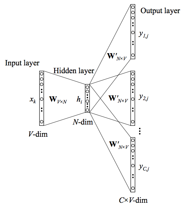
In the above model \(\mathbf{x}\) represents the one-hot encoded vector corresponding to the input word in the training instance and \(\{\mathbf{y_1},...\mathbf{y_C}\}\) are the one-hot encoded vectors corresponding to the output words in the training instance. The \(V \times N\) matrix \(\mathbf{W}\) is the weight matrix between the input layer and hidden layer whose \(i^{th}\) row represents the weights corresponding to the \(i^{th}\) word in the vocabulary. This weight matrix \(\mathbf{W}\) is what we are interested in learning because it contains the vector encodings of all of the words in our vocabulary (as its rows). Each output word vector also has an associated \(N \times V\) output matrix \(\mathbf{W'}\). There is also a hidden layer consisting of \(N\) nodes (the exact size of \(N\) is a training parameter).
From my previous blog post, we know that the input to a unit in the hidden layer \(h_i\) is simply the weighted sum of its inputs. Since the input vector \(\mathbf{x}\) is one-hot encoded, the weights coming from the nonzero element will be the only ones contributing to the hidden layer. Therefore, for the input \(\mathbf{x}\) with \(x_k=1\) and \(x_{k'}=0\) for all \(k' \neq k\) the outputs of the hidden layer will be equivalent to the \(k^{th}\) row of \(\mathbf{W}\). Or mathematically,
\[\mathbf{h}=\mathbf{x}^T \mathbf{W}=\mathbf{W}_{(k, .)} := \mathbf{v}_{w_I}\]Notice that there is no activation function used here. This is presumably because the inputs are bounded by the one-hot encoding. In the same way, the inputs to each of the \(C \times V\) output nodes is computed by the weighted sum of its inputs. Therefore, the input to the \(j^{th}\) node of the \(c^{th}\) output word is
\[u_{c,j}=\mathbf{v'}_{w_j}^T \mathbf{h}\]However we can also observe that the output layers for each output word share the same weights therefore \(u_{c,j}=u_j\). We can finally compute the output of the \(j^{th}\) node of the \(c^{th}\) output word via the softmax function which produces a multinomial distribution
\[p(w_{c,j}=w_{O,c} | w_I)=y_{c,j}=\frac{exp(u_{c,j})}{\sum_{j'=1}^V exp(u_{j'})}\]In plain english, this value is the probability that the output of the \(j^{th}\) node of the \(c^{th}\) output word is equal to the actual value of the \(j^{th}\) index of the \(c^{th}\) output vector (which is one-hot encoded).
Learning the Weights with Backpropagation and Stochastic Gradient Descent
Now that we know how inputs are propograted forward through the network to produce outputs, we can derive the error gradients necessary for the backpropagation algorithm which we will use to learn both $\mathbf{W}$ and \(\mathbf{W'}\). The first step in deriving the gradients is defining a loss function. This loss function will be
\[\begin{align} E &= -\log p(w_{O,1}, w_{O,2}, ..., w_{O,C} | w_I) \\ &= -\log \prod^C_{c=1} \frac{exp(u_{c,j^*_c})}{\sum^V_{j'=1} exp(u_j')} \\ &= -\sum^C_{c=1}u_{j^*_c} +C \cdot \log \sum^V_{j'=1} exp(u_{j'}) \end{align}\]which is simply the probability of the output words (the words in the input word’s context) given the input word. Here, \(j^*_c\) is the index of the \(c^{th}\) output word. If we take the derivative with respect to \(u_{c,j}\) we get
\[\frac{\partial{E}}{\partial{u_{c,j}}}=y_{c,j}-t_{c,j}\]where \(t_{c,j}=1\) if the \(j^{th}\) node of the \(c^{th}\) true output word is equal to \(1\) (from its one-hot encoding), otherwise \(t_{c,j}=1\). This is the prediction error for node \(c,j\) (or the \(j^{th}\) node of the \(c^{th}\) output word).
Now that we have the error derivative with respect to inputs of the final layer, we can derive the derivative with respect to the output matrix \(\mathbf{W'}\). Here we use the chain rule
\[\begin{align} \frac{\partial E}{\partial w'_{ij}} &=\sum^C_{c=1} \frac{\partial E}{\partial u_{c,j}} \cdot \frac{\partial u_{c,j}}{\partial w'_{ij}} \\ &=\sum^C_{c=1} (y_{c,j}-t_{c,j}) \cdot h_i \end{align}\]Therefore the gradient descent update equation for the output matrix \(\mathbf{W'}\) is
\[w'^{(new)}_{ij} =w'^{(old)}_{ij}- \eta \cdot \sum^C_{c=1} (y_{c,j}-t_{c,j}) \cdot h_i\]Now we can derive the update equation for the input-hidden layer weights in \(\mathbf{W}\). Let’s start by computing the error derivative with respect to the hidden layer.
\[\begin{align} \frac{\partial{E}}{\partial{h_i}} &=\sum^V_{j=1} \frac{\partial{E}}{\partial{u_j}} \cdot \frac{\partial{u_j}}{\partial{h_i}} \\ &=\sum^V_{j=1} \sum^C_{c=1} (y_{c,j}-t_{c,j}) \cdot w'_{ij} \end{align}\]Now we are able to compute the derivative with respect to \(\mathbf{W}\)
\[\begin{align} \frac{\partial{E}}{\partial{w_{ki}}} &=\frac{\partial{E}}{\partial{h_i}} \cdot \frac{\partial{h_i}}{\partial{w_{ki}}} \\ &= \sum^V_{j=1} \sum^C_{c=1} (y_{c,j}-t_{c,j}) \cdot w'_{ij} \cdot x_k \end{align}\]and finally we arrive at our gradient descent equation for our input weights
\[w^{(new)}_{ij} =w^{(old)}_{ij}- \eta \cdot \sum^V_{j=1} \sum^C_{c=1} (y_{c,j}-t_{c,j}) \cdot w'_{ij} \cdot x_j\]As you can see, each gradient descent update requires a sum over the entire vocabulary \(V\) which is computationally expensive. In practice, computation techniques such as hierarchical softmax and negative sampling are used to make this computation more efficient.