Calling CUDA from Python to Speed Up Linear Algebra
Numpy is the go-to library for linear algebra computations in python. It is a highly optimized library that uses BLAS as well as SIMD vectorization resulting in very fast computations. Having said that, there are times when it is preferable to perform linear algebra computations on the GPU i.e. using CUDA’s cuBLAS linear algebra library. For example, the linear algebra computations associated with training large deep neural networks are commonly performed on GPU. In cases like these, the vectors and matrices are so large that the parallelization offerred by GPUs allows them to outperform linear algebra libraries like numpy.
The purpose of this blog post is two-fold.
- To show how you can call compiled cuBLAS code from python to improve the performance of linear algebra computations and
- To identify the point at which this cuBLAS code starts to outperform numpy.
The environment I am using for the code in this blog post is Ubuntu 16.04 LTS, with CUDA 10 and a GTX 980M GPU.
Calling Compiled cuBLAS Code from Python
Let’s start with a simple function that calls cuBLAS’s cublasSgemm() which is a single precision matrix multiplication.
void run(ftype *i1, ftype  *i2, ftype *o1, int d){

	ftype *d_i1, *d_i2, *d_o1;
	int ds = d*d*sizeof(ftype);
	cudaMalloc(&d_i1, ds);
	cudaMalloc(&d_i2, ds);
	cudaMalloc(&d_o1, ds);
	cudaMemcpy(d_i1, i1, ds, cudaMemcpyHostToDevice);
	cudaMemcpy(d_i2, i2, ds, cudaMemcpyHostToDevice);

	cublasHandle_t h;
	cublasCreate(&h);
	ftype alpha = 1.0;
	ftype beta = 0.0;
	cublasSgemm(h, CUBLAS_OP_N, CUBLAS_OP_N, d, d, d, &alpha, d_i1, d, d_i2, d, &beta, d_o1, d);
	cudaMemcpy(o1, d_o1, ds, cudaMemcpyDeviceToHost);

	cudaFree(d_i1);
	cudaFree(d_i2);
	cudaFree(d_o1);
}
The function takes pointers to the two input matrices (as arrays in column-major format) and an additional matrix which is reserved for the result. Within the function we must allocate memory on the device for each matrix as well as copy the two input matrices onto the device. After cublasSgemm() is called we copy the result back onto the host and clean up our memory. We can then compile this code into a shared object file called cublas_test.so with the nvcc compiler using the following command.
nvcc cublas_test.cu -o cublas_test.so -shared -Xcompiler -fPIC -lcublas
The next step is to call this shared object file from python. We can do this with python’s ctypes library.
E = ctypes.cdll.LoadLibrary("cublas_test.so")

N = matrix_dim * matrix_dim

m1 = numpy.ones((N), dtype=numpy.float32)
m2 = numpy.ones((N), dtype=numpy.float32)
output_m = numpy.zeros((N), dtype=numpy.float32)

E.run(ctypes.c_void_p(m1.ctypes.data),
      ctypes.c_void_p(m2.ctypes.data),
      ctypes.c_void_p(output_m.ctypes.data),
      ctypes.c_int(matrix_dim))
The first line loads the shared object file, then we initialize our two input matrices as column-major vectors (this is the only format cublasSgemm() accepts) as well as the result matrix. We then call the run() function from our loaded shared object file which we supply with our inputs. The resulting matrix can then be found in the output_m variable. And this is how we call cuBLAS from python!
When does cuBLAS Outperform Numpy?
Now that we can successfully call cuBLAS from python, let’s see how it performs compared to numpy. The benefits of parallelization only shine through when there is enough data to take advantage of it. Otherwise the benefits are cancelled out by the overhead associated thread organization and data transfer. Therefore, we would expect numpy to outperform cuBLAS for smaller input matrices but there should be an point at which the matrices become large enough for cuBLAS’s parallelization to overtake numpy.
The code used for this experiment can be found here, but basically we are just timing the matrix multiplication operations for cuBLAS and numpy for increasing input matrix sizes. Below are the timing functions for each implementation.
def cublas_mm(matrix_dim):
    N = matrix_dim * matrix_dim

    m1 = numpy.ones((N), dtype=numpy.float32)
    m2 = numpy.ones((N), dtype=numpy.float32)
    output_m = numpy.ones((N), dtype=numpy.float32)

    t0 = time.time()

    E.run(ctypes.c_void_p(m1.ctypes.data),
          ctypes.c_void_p(m2.ctypes.data),
          ctypes.c_void_p(output_m.ctypes.data),
          ctypes.c_int(matrix_dim))

    t1 = time.time()
    return t1 - t0


def numpy_mm(matrix_dim):
    m1 = numpy.ones((matrix_dim, matrix_dim), dtype=numpy.float32)
    m2 = numpy.ones((matrix_dim, matrix_dim), dtype=numpy.float32)

    t0 = time.time()

    _ = numpy.dot(m1, m2)

    t1 = time.time()
    return t1 - t0
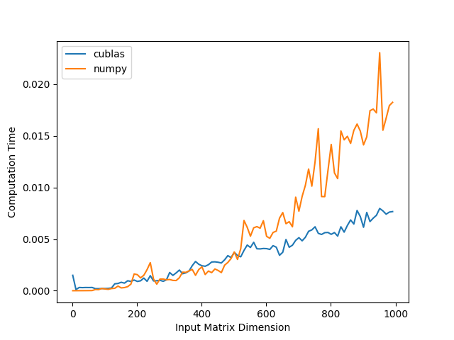
The times can be a bit volatile so we average over 100 computations for each matrix dimension. Below is a plot of the timing results.

As we expected, numpy is slightly faster for smaller input matrices but for matrices larger than around 500 rows and columns cuBLAS starts to become much faster. Of course these results are highly environment-dependent but the general pattern should hold.
The code used in this post can be found in this github repo. Thank you for reading.