Named Entity Recognition with RNNs in TensorFlow
Many tutorials for RNNs applied to NLP using TensorFlow are focused on the language modelling problem. But another interesting NLP problem that can be solved with RNNs is named entity recognition (NER). This blog post will cover how to train a LSTM model in TensorFlow in the context of NER - all code mentioned in this post can be found in an associated Colab notebook.
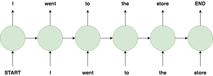
Both language modelling and NER use a many-to-many RNN architecture where each input has a corresponding output, however they differ in what the outputs are. With language modelling, an input is a word in a sentence and the corresponding output is the next word in the sentence - so one training example consists of a list of words in a sentence as the input and that same sentence right-shifted by one word as the output.
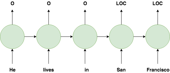
With NER, an input is a word in a sentence and the corresponding output is that word’s label. In the below example, words corresponding to locations are given the “LOC” label and non-entity words are given the “O” label.
The output space for the NER problem is much smaller than the output space for the language modelling problem (which is the same as the input space). With NER, words corresponding to entities of interest are typically far less common than non-entity words (i.e. those labelled as “O”), therefore NER suffers from the class imbalance problem.
In the diagrams above, each input is shown as a word, however, RNNs can also work with character inputs. Certain entities (i.e. people’s names) contain distinctive character sequences which makes a character-based RNN better equipped to learn those patterns so we are going to use a character-based RNN here.
The Data
This github repository holds a great collection of NER training data. In this post, we’ll use the CONLL2003 dataset which is of the following form
EU NNP B-NP B-ORG
rejects VBZ B-VP O
German JJ B-NP B-MISC
call NN I-NP O
to TO B-VP O
boycott VB I-VP O
British JJ B-NP B-MISC
lamb NN I-NP O
. . O O
where the left-most column contains tokens and the other columns are the corresponding entities. For this post we will only look at the right-most column entities - these will be our outputs. Each sentence is separated by an empty line. There are 14,985 total sentences in the training set and 9 entity labels which are
{'I-ORG', 'B-PER', 'I-MISC', 'B-LOC', 'I-PER', 'O', 'I-LOC', 'B-ORG', 'B-MISC'}
There is also a validation and test set.
Preprocessing
Before we train the model, we need to transform the raw dataset into a form that a character-based RNN can understand. The first step is to separate the raw dataset into the input words and the output entities and split them by character so the first example would look like
[['E','U',' ','r','e','j','e','c','t','s',...,'l','a','m','b','.'],['B-ORG','B-ORG','O','O','O','O','O','O','O','O',...,'O','O','O','O','O']]
The next step is to map every character to an id and every entity to an id such that each example would look something like
[[36,22,19,12,5,24,5,67,13,15,...,52,26,45,32,20],[4,4,1,1,1,1,1,1,1,1,... ,1,1,1,1,1]]
The final dataset is a sequence of these input/output tuples. The dataset can be fed to the model during training time with a generator such as
def gen_train_series():

    for eg in training_data:
        yield eg[0],eg[1]
and the generator can be fed in batches with
BATCH_SIZE = 128

series = tf.data.Dataset.from_generator(gen_train_series,output_types=(tf.int32, tf.int32),output_shapes = ((None, None)))

ds_series_batch = series.shuffle(BUFFER_SIZE).padded_batch(BATCH_SIZE, padded_shapes=([None], [None]), drop_remainder=True)
where, for computational reasons, each batch is padded with zeros (with .padded_batch()) such that all inputs and outputs are of the same length. One batch of inputs will look something like
tf.Tensor(
[[34 49 40 ...  0  0  0]
 [43 46 45 ...  0  0  0]
 [54 65 79 ...  0  0  0]
 ...
 [ 3  1 36 ...  0  0  0]
 [40 66  1 ...  0  0  0]
 [35 81 78 ...  0  0  0]], shape=(128, 228), dtype=int32)
and one batch of ouputs will look something like
tf.Tensor(
[[2 2 2 ... 0 0 0]
 [3 3 3 ... 0 0 0]
 [5 5 5 ... 0 0 0]
 ...
 [2 2 2 ... 0 0 0]
 [2 2 2 ... 0 0 0]
 [8 8 8 ... 0 0 0]], shape=(128, 228), dtype=int32)
Notice the character id’s in the input batch and the class id’s in the output batch and the trailing zeros in both which are the padding. These steps are applied to the training, validation and test sets.
The Model
The model will use an LSTM architecture beginning with an embedding layer. Rather than using pre-trained embeddings or training them separately, the embeddings will be trained alongside the main LSTM model. Also, aside from the LSTM layer there is a final full-connected layer that produces the predictions. The model is created in tensorflow with the following code.
  vocab_size = len(vocab)+1

  # The embedding dimension
  embedding_dim = 256

  # Number of RNN units
  rnn_units = 1024

  label_size = len(labels)

  def build_model(vocab_size,label_size, embedding_dim, rnn_units, batch_size):
        model = tf.keras.Sequential([
            tf.keras.layers.Embedding(vocab_size, embedding_dim,
                              batch_input_shape=[batch_size, None],mask_zero=True),
            tf.keras.layers.LSTM(rnn_units,
                        return_sequences=True,
                        stateful=True,
                        recurrent_initializer='glorot_uniform'),
            tf.keras.layers.Dense(label_size)
            ])
        return model

  model = build_model(
        vocab_size = len(vocab)+1,
        label_size=len(labels)+1,
        embedding_dim=embedding_dim,
        rnn_units=rnn_units,
        batch_size=BATCH_SIZE)
It is also important to notice the mask_zero=True argument in the embedding layer - this tells the model that the zeros in the input and output batches are just padding rather than legitimate character or class ids. We can get a nice overview of the model we just defined using model.summary() which returns
_________________________________________________________________
Layer (type)                 Output Shape              Param #
=================================================================
embedding_1 (Embedding)      (128, None, 256)          22272
_________________________________________________________________
lstm_1 (LSTM)                (128, None, 1024)         5246976
_________________________________________________________________
dense_1 (Dense)              (128, None, 10)           10250
=================================================================
Total params: 5,279,498
Trainable params: 5,279,498
Non-trainable params: 0
_________________________________________________________________
Finally we need to define the loss function and the optimization algorithm we will use during training. Since our output classes are integers, we will use sparse_categorical_crossentropy as our loss function.
def loss(labels, logits):
    return tf.keras.losses.sparse_categorical_crossentropy(labels, logits, from_logits=True)
Also, we’ll use the ADAM optimization algorithm for training and with the metrics argument tell the model to report the accuracy at each training iteration.
model.compile(optimizer='adam', loss=loss, metrics=[tf.keras.metrics.SparseCategoricalAccuracy()])
Now we can actually train the model which can be done with
EPOCHS=20

history = model.fit(ds_series_batch, epochs=EPOCHS, validation_data=ds_series_batch_valid)
Here we have chosen to train the model over 20 epochs of the training set and at each epoch validate the model against out validation set.
The training output will look something like
Epoch 1/20
117/117 [==============================] - 62s 533ms/step - loss: 0.2124 - sparse_categorical_accuracy: 0.7984 - val_loss: 0.0000e+00 - val_sparse_categorical_accuracy: 0.0000e+00
Epoch 2/20
117/117 [==============================] - 56s 476ms/step - loss: 0.1219 - sparse_categorical_accuracy: 0.8455 - val_loss: 0.1149 - val_sparse_categorical_accuracy: 0.8524
Epoch 3/20
117/117 [==============================] - 56s 477ms/step - loss: 0.1009 - sparse_categorical_accuracy: 0.8671 - val_loss: 0.0996 - val_sparse_categorical_accuracy: 0.8731
Epoch 4/20
117/117 [==============================] - 56s 476ms/step - loss: 0.0890 - sparse_categorical_accuracy: 0.8828 - val_loss: 0.0921 - val_sparse_categorical_accuracy: 0.8835
Epoch 5/20
117/117 [==============================] - 56s 477ms/step - loss: 0.0824 - sparse_categorical_accuracy: 0.8918 - val_loss: 0.0848 - val_sparse_categorical_accuracy: 0.8942
Epoch 6/20
117/117 [==============================] - 56s 478ms/step - loss: 0.0779 - sparse_categorical_accuracy: 0.8975 - val_loss: 0.0814 - val_sparse_categorical_accuracy: 0.8986
Epoch 7/20
117/117 [==============================] - 56s 479ms/step - loss: 0.0725 - sparse_categorical_accuracy: 0.9035 - val_loss: 0.0785 - val_sparse_categorical_accuracy: 0.9030
Epoch 8/20
117/117 [==============================] - 56s 476ms/step - loss: 0.0710 - sparse_categorical_accuracy: 0.9071 - val_loss: 0.0759 - val_sparse_categorical_accuracy: 0.9057
Epoch 9/20
117/117 [==============================] - 56s 478ms/step - loss: 0.0669 - sparse_categorical_accuracy: 0.9119 - val_loss: 0.0740 - val_sparse_categorical_accuracy: 0.9095
Epoch 10/20
117/117 [==============================] - 56s 479ms/step - loss: 0.0634 - sparse_categorical_accuracy: 0.9163 - val_loss: 0.0725 - val_sparse_categorical_accuracy: 0.9116
Epoch 11/20
117/117 [==============================] - 56s 477ms/step - loss: 0.0600 - sparse_categorical_accuracy: 0.9217 - val_loss: 0.0695 - val_sparse_categorical_accuracy: 0.9152
Epoch 12/20
117/117 [==============================] - 56s 478ms/step - loss: 0.0561 - sparse_categorical_accuracy: 0.9262 - val_loss: 0.0683 - val_sparse_categorical_accuracy: 0.9176
Epoch 13/20
117/117 [==============================] - 56s 476ms/step - loss: 0.0526 - sparse_categorical_accuracy: 0.9307 - val_loss: 0.0657 - val_sparse_categorical_accuracy: 0.9210
Epoch 14/20
117/117 [==============================] - 56s 476ms/step - loss: 0.0499 - sparse_categorical_accuracy: 0.9355 - val_loss: 0.0667 - val_sparse_categorical_accuracy: 0.9212
Epoch 15/20
117/117 [==============================] - 56s 477ms/step - loss: 0.0457 - sparse_categorical_accuracy: 0.9402 - val_loss: 0.0658 - val_sparse_categorical_accuracy: 0.9226
Epoch 16/20
117/117 [==============================] - 56s 478ms/step - loss: 0.0414 - sparse_categorical_accuracy: 0.9459 - val_loss: 0.0644 - val_sparse_categorical_accuracy: 0.9257
Epoch 17/20
117/117 [==============================] - 56s 478ms/step - loss: 0.0381 - sparse_categorical_accuracy: 0.9506 - val_loss: 0.0660 - val_sparse_categorical_accuracy: 0.9248
Epoch 18/20
117/117 [==============================] - 56s 475ms/step - loss: 0.0354 - sparse_categorical_accuracy: 0.9541 - val_loss: 0.0652 - val_sparse_categorical_accuracy: 0.9274
Epoch 19/20
117/117 [==============================] - 56s 475ms/step - loss: 0.0321 - sparse_categorical_accuracy: 0.9586 - val_loss: 0.0659 - val_sparse_categorical_accuracy: 0.9294
Epoch 20/20
117/117 [==============================] - 56s 475ms/step - loss: 0.0364 - sparse_categorical_accuracy: 0.9542 - val_loss: 0.0644 - val_sparse_categorical_accuracy: 0.9300
As you can see, by the last epoch the validation accuracy reaches 93% which seems very good however with class imbalanced classification problems such as this one accuracy can be a deceptive evaluation metric.
Evaluation
In order to better evaluate our trained model we will use the held-out test set and we will use a more rigorous evaluation metric. To get a more complete evaluation we can look at the confusion matrix for the test set.
[[  6377    177     29    502     38     56     91     43    109]
 [   162 187279    929    360    857   2132    150   1006    266]
 [    15    595   7002     45    794   1795      6    558      0]
 [   405    547     70   3110     18     53    136     89    124]
 [    10    287    623     46   1983    641      6    167     37]
 [    14    609    881     93    656   4273     13    629      8]
 [   142     93      5    275      6     14    863     13     66]
 [    91    743    893     73    460   1186     21   6551     23]
 [    61    190     17    229     25     12     86      7    377]]
We can also use the scikit classification_report which displays the precision, recall and f1-score for each output class.
              precision    recall  f1-score   support

         1.0       0.88      0.86      0.87      7422
         2.0       0.98      0.97      0.98    193141
         3.0       0.67      0.65      0.66     10810
         4.0       0.66      0.68      0.67      4552
         5.0       0.41      0.52      0.46      3800
         6.0       0.42      0.60      0.49      7176
         7.0       0.63      0.58      0.61      1477
         8.0       0.72      0.65      0.69     10041
         9.0       0.37      0.38      0.37      1004

    accuracy                           0.91    239423
   macro avg       0.64      0.65      0.64    239423
weighted avg       0.92      0.91      0.91    239423
As you can see, this shows a slightly different picture than the 93% validation accuracy. The support column shows the number of examples corresponding to each output class in the test set. The most common class (the “O”’s) has a very high precision and recall which bumps up the overall accuracy considerably. However if you look at some of the other classes the precision and recall are much lower. This is typical of the class imbalance problem where the model focuses on learning the over-represented class often at the expense of the under-represented class. There are a few ways to fix this such as over-sampling the under-represented classes or under-sampling the over-represented classes in the training set - but that is beyond the scope of this blog post. Another future direction is to try a bidirectional LSTM model which could improve results.
Thank you for reading.