The Kalman filter is a popular model that can use measurements from multiple sources to track an object in a process known as sensor fusion. This post will cover two sources of measurement data - radar and lidar. It will also cover an implementation of the Kalman filter using the TensorFlow framework. It might surprise some to see TensorFlow being used outside of a deep learning context, however here we are exploiting TensorFlow’s linear algebra capabilies which will be needed in the Kalman filter implementation. Additionaly, if you have tensorflow-gpu installed, TensorFlow can allow us to put GPUs behind our linear algebra computations which is a nice bonus. The code corresponding to this post can be found here.

Radar and Lidar Data

Lidar captures data in the form of a point cloud. So we are pretending that the position of the object we are tracking has been extracted from the lidar’s point cloud (that process is beyond the scope of this blog post). So a lidar measurement will be a vector of the form

where \(p_x\) and \(p_y\) are the x and y positions of the object. Radar, on the other hand, is able to measure both position and velocity (through the doppler effect). So a radar measurement will be a vector of the form

where \(\rho\), \(\phi\) and \(\dot{\rho}\) are the range (distance to the object), bearing (direction of the object relative to the sensor) and radial velocity (rate of change of range), respectively. Radar’s positional measurements are generally less accurate than lidar’s however radar is also able to measure velocity which lidar cannot - so you can see how these two measurement devices complement each other and tend to be used alongside each other.

Kalman Filters

Now let’s explain the Kalman filter. We will start with some intuition, then we will learn the general setup, then we will see how Kalman filters can be used with radar and lidar data.

The Intuition

All measurement devices have inherent uncertainty associated with their measurements (usually the device manufacturer quantifies this uncertainty for us). The intuition is that if you have

1. past measurement data of where the object was and
2. understand the movement dynamics of the object

then you can predict where the object will be at the next time step. The Kalman filter says that if you combine the predicted location of the object at the next time step with the actual measurement of the object at that timestep then you can improve upon the measurement error. The idea is that if the measurement of an object is close to where you predicted it to be then you can be more certain of that measurement than a measurement that is far from where you predicted it to be. So basically the Kalman filter is an iterative 2-step process where when a new measurement is observed

1. A prediction step is performed
2. An update step is performed where we update our estimate of the object's location by comparing the prediction to the actual measurement.

The Setup

Here we will be considering the 2-D case where velocity is assumed to be constant. The state vector consists of the x and y positions of the object as well as the x and y velocities.

Assuming a linear motion model we can predict the position at the next time step in one dimension with

and in matrix form this is

and since we are assuming constant velocity, the velocity update \(v'\) is no different from the original \(v\). This is called the prediction step of the Kalman filter and takes the general form

where \(F\) is called the process matrix which defines the prediction process. In our case it was

But we are also interested in the uncertainty relating to our state vector estimate. We can model this with a covariance matrix \(P\) that can also be predicted given the previous covariance matrix with

where \(Q\) is the process covariance matrix.

So now we have our predicted state vector \(x'\) after a time step of \(\Delta t\) and we also have the meausurement \(z\). In the update step we use \(z\) to improve our state vector estimate \(x'\). The first step is to convert the state vector into the measurement space using with

where the matrix \(H\) determines the conversion. We will see later that since radar and lidar measure different things, they each have different measurement spaces which requires different \(H\) matrices. \(z'\) is often called the predicted measurement since it is the predicted state vector projected into the measurement space. Then next step is to compare the predicted measurement with the actual measurement with

The final part is to actually update the state vector \(x\) and the state covariance \(P\) - the following is presented without proof but feel free to look up the derivation if you are interested.

So we have essentially gone through one iteration (the prediction step and update step) of a Kalman filter when a measurement is observed. Next we’ll see how the prediction and update steps work specifically for radar and lidar data.

The Radar and Lidar Prediction Step

The prediction step does not depend on the measurement so it is the same for both radar and lidar. We simply extend the prediction equations from the last section to 2 dimensions so now

and, again, the state covariance prediction is

The Lidar Update Step

The lidar updates step is quite straight-forward. As stated previously, lidar only measures position in the form

For this reason, in order to project the state vector \(x\) into the measurement space, the x and y velocities are removed by the \(H\) matrix which is of the form

The rest of the update steps follow directly from the last section.

The Radar Update Step

The radar update step is more complicated. As stated previously, the radar measurement is of the form

Unlike the lidar case, it is not immediately obvious how to project our state vector (which contains positions and linear velocities) into this measurement space. It turns out that the way to do this is

which is presented without proof. However, this presents a problem because, unlike the lidar case, this is a nonlinear transformation. Since we never actually derived the Kalman filter from first principles it is not immediately obvious why this is a problem. The Kalman filter assumes that \(z'\) will be Gaussian. Passing a Gaussian distribution through a linear function also results in a Gaussian however passing a Gaussian distribution through a nonlinear function may not result in a Gaussian - so this projection won’t work.

One way to solve this problem is to compute a linear approximation by performing a multivariate Taylor series expansion on \(h\) around \(x'\) - in this way the result will remain Gaussian. Again this is presented without proof but this requires computing the matrix of partial derivatives of \(z_{radar}\) with respect to \(x\) (also known as the Jacobian) and using it as our \(H\) matrix for radar measurements which turns out to be

Also, unlike the lidar case, this matrix needs to be recomputed at each iteration since the state vector is changing. The rest of the update steps remain the same.

The Sensor Fusion Procedure

The idea behind sensor fusion is to asynchronously receive radar and lidar measurements and use both to update our state vector estimate \(x\) using the Kalman filter procedure we just learned. The following diagram explains the general flow.

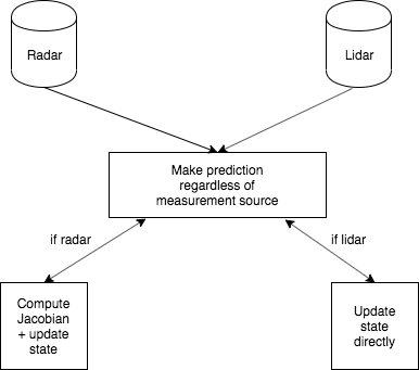
First, when any measurement is received, a state and state covariance prediction is made. Then the update step is performed according to the measurement type. If it is a lidar measurement, the update step is performed directly using the prediction and the static \(H\) matrix. If it is a radar measurement, the Jacobian is computed which serves as the \(H\) matrix and then the update is preformed. This is repeated for each measurement.

TensorFlow Implementation

Finally, let’s implement this procedure in TensorFlow (the full code can be found here). The prediction step is implemented simply with

self.x = tf.matmul(self.F, self.x)
self.P = tf.matmul(tf.matmul(self.F, self.P), tf.transpose(self.F)) + self.Q

The lidar measurement prediction is performed with

z_pred = tf.matmul(self.H_lidar, self.x)

and the radar measurement prediction is performed with

px, py, vx, vy = self.x.numpy()
h_np = [np.sqrt(px[0] * px[0] + py[0] * py[0]), np.arctan2(py[0], px[0]),
                (px[0] * vx[0] + py[0] * vy[0]) / np.sqrt(px[0] * px[0] + py[0] * py[0])]

In the radar update step the Jacobian can be computed with

px, py, vx, vy = self.x.numpy()

d1 = px[0] * px[0] + py[0] * py[0]
d2 = np.sqrt(d1)
d3 = d1 * d2

H = tf.convert_to_tensor(
        [[px[0] / d2, py[0] / d2, 0, 0], 
        [-(py[0] / d1), px[0] / d1, 0, 0],
         [py[0] * (vx[0] * py[0] - vy[0] * px[0]) / d3, px[0] * (px[0] * vy[0] - py[0] * vx[0]) / d3, px[0] / d2, py[0] / d2]]
            , dtype=tf.float32
    )

Finally the full update step can performed with

if z_.device == Device.radar:
    z_pred = self.radar_measurement_prediction()
    H = self.compute_jacobian()
    R = self.R_radar
    y = z - z_pred

elif z_.device == Device.lidar:
    z_pred = self.lidar_measurement_prediction()
    H = self.H_lidar
    R = self.R_lidar
    y = z - z_pred

S = tf.matmul(tf.matmul(H, self.P), tf.transpose(H)) + R
K = tf.matmul(tf.matmul(self.P, tf.transpose(H)), tf.linalg.inv(S))

self.x = self.x + tf.matmul(K, y)
x_len = self.x.get_shape()[0]
I = tf.eye(x_len, x_len)
self.P = tf.matmul((I - tf.matmul(K, H)), self.P)

A full demo for this implementation using simulated radar and lidar measurements can be found here.

Problems with this Approach

The main problem with this approach is that the linear motion model does not work well for tracking objects that do not move in a linear fashion. For example, if you are tracking a turning car, the prediction will consistently over-shoot because the model is assuming that the car is always moving in a straight line. Incorporating more flexible motion models and turn information can help with this.

Thank you for reading.

References

• code from this post
• Kalman Filter